These symmetry relations hold:
where
Si
(
−z
)
=−Si
(
z
)
Ci
(
−z
)
= Ci
(
z
)
− i✜ 0 < arg
(
z
)
< ✜
where
✏ = 0.577215664901533 (Euler’s constant)
Si(x) approaches as , and Ci(x) approaches 0 as . These series expansions also calculate
✜/2 x
d∞
x
d∞
the integrals:
Si
(
z
)
=
✟
n=0
∞
(
−1
)
n
z
2n+1
(
2n+1
)(
2n+1
)
!
Ci
(
z
)
= ✏ + ln
(
z
)
+
✟
n=1
∞
(
−1
)
n
z
2n
2n
(
2n
)
!
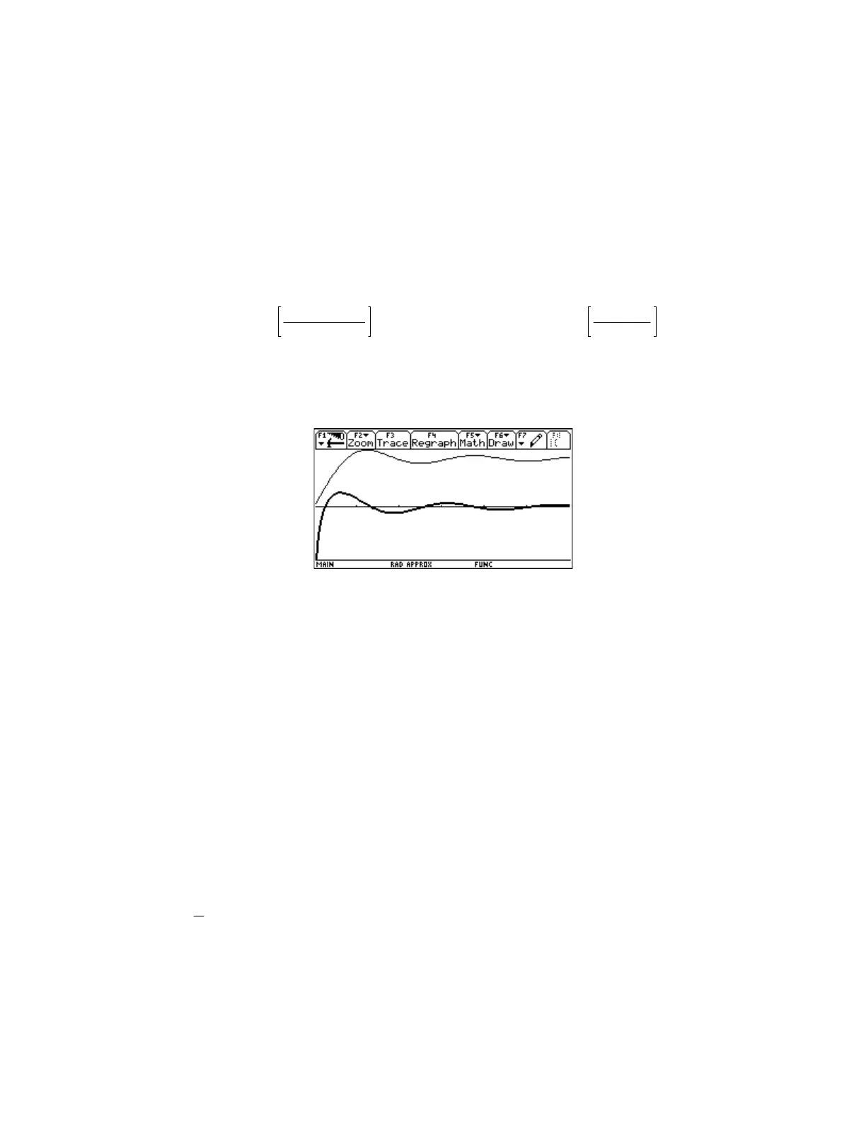
This plot show the two functions from x = 0.1 to x = 15. The thin plot trace is Si(x), and the thick trace is
Ci(x).
These functions can be calculated with the routines Si() and Ci(), shown below. These routines are not
terribly accurate, but are good enough for most engineering applications. For arguments less than ,
✜
the built-in nint() function is used to integrate the function definition. For arguments greater than , a
✜
rational approximation is used. The transition point of was selected more for reasons of execution
✜
time than anything else. Above that point, nint() takes significantly longer to execute.
The routines must be installed in a folder called /spfn. Set the modes to Approx, and Rectangular or
Polar complex before execution. Input arguments must be real numbers, not complex numbers. Note
that Ci(x) returns a complex number for arguments less than zero.
Because different methods are used for different argument ranges, there is a discontinuity in the
function at . The discontinuity is about 2.6E-7 for Si(x), and about 1.5E-8 for Ci(x). This may not
x = ✜
practically affect the results when simply evaluating the function, but it may be a problem if you
numerically differentiate the functions, or try to find a maximum or minimum with the functions.
The rational approximations used for Si(x) and Ci(x) are based on the identities
Si
(
x
)
=
✜
2
− f
(
x
)
cos
(
x
)
− g
(
x
)
sin
(
x
)
Ci
(
x
)
= f
(
x
)
sin
(
x
)
− g
(
x
)
cos
(
x
)
where
6 - 62
 Loading...