Instruction Manual Easygraph
Page 33
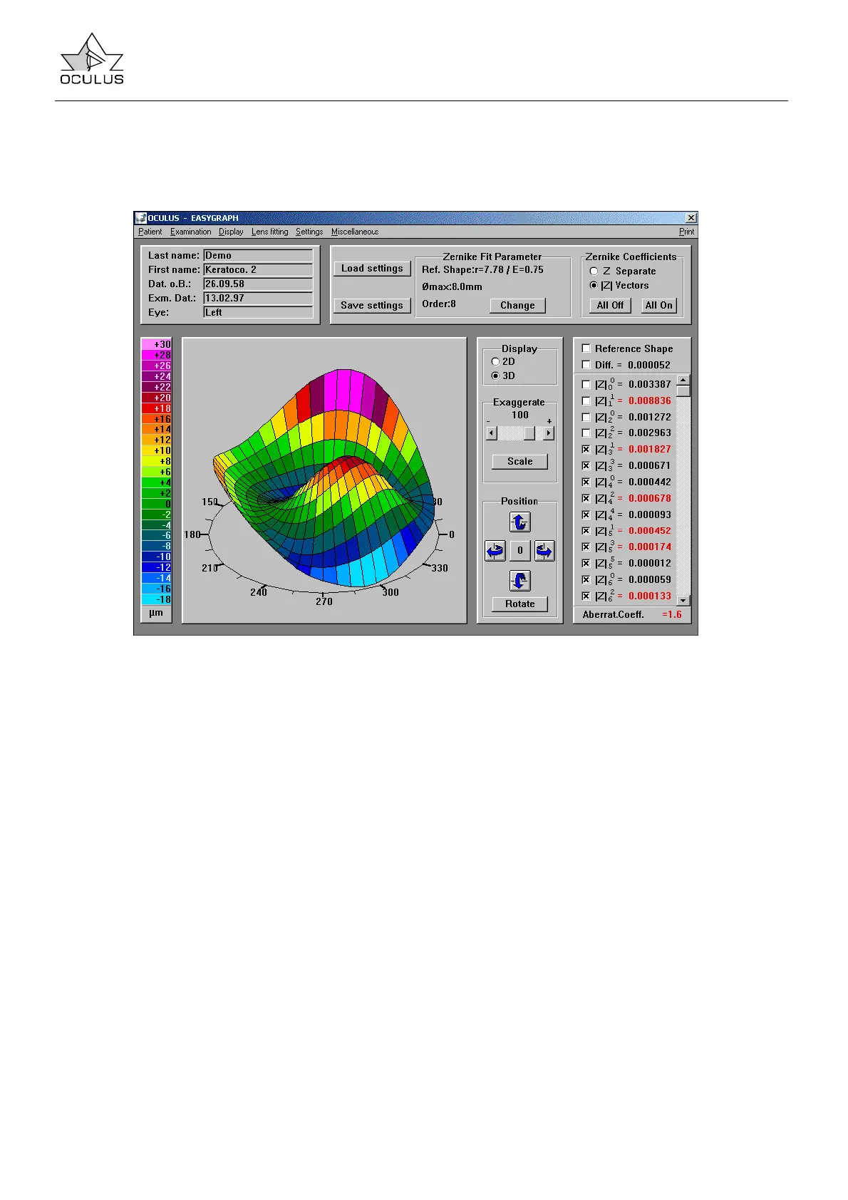
7.5.2.5.2 Zernike Analysis Using the Easygraph
The Easygraph performs a Zernike analysis on
measured height data. It calculates for each Zernike
polynomial a coefficient which describes the
contribution of that polynomial to the height data.
To start the Zernike analysis select “Zernike
analysis” under the menu bar function “Display”.
After the calculation of all Zernike coefficients has
been carried out, the following display appears:
On the left side there appears a three-dimensional
image representing all Zernike polynomials that have
been activated. This display is scaled automatically
when it is generated. It can also be rotated manually
using the buttons in the “Position” field. Clicking the
“Rotate” button causes the 3D image to rotate
continuously until a new task is activated.
The color bar on the left shows which color
corresponds to which height value.
The Zernike coefficients are listed on the right. A
scroll bar permits scrolling the list up and down in the
case of more than 14 coefficients.
Polynomials can be individually activated or
deactivated by clicking the corresponding check
boxes.
Activating or deactivating Zernike polynomials
immediately causes the 3D image to be redrawn.
The new image is not scaled automatically in this
case but is shown in same scale as the previous
image. This makes it easier to assess the effects that
individual polynomials have on the image. By clicking
the “Scale” button the image may be displayed in a
scale optimal for it. In addition, the scale may be
manually adjusted using the “Exaggerate” slider
control.
At the top right is a field titled “Zernike
Coefficients” which provides the option of viewing
the Zernike coefficients in the “Z Separate” or the
“|Z| Vectors” display mode. Normally one Zernike
component consists of two polynomials (e.g. Z 2,2
and Z 2,-2 for the astigmatic component). These two
terms only differ by a trigonometric component (Z 2,2
contains a cosine function and Z 2,-2 a sine
function):
z2,2(r,phi) =Z2,2*SQR(6) * ( 1*r^2 ) * COS(2*phi)
z2,-2(r,phi)=Z2,-2* SQR(6) * ( 1*r^2 ) * SIN(2*phi)
The two terms of the astigmatic component have a
phase difference of 45°, as one can infer from the
“Z Separate” mode. The angle resulting from the
combined polynomial, however, is determined by the
ratio between the coefficients of Z 2,2 and Z 2,-2. A
more intuitive approach results from a combination of
the two polynomials and, instead of separate sine
and cosine terms, the computation of the length and
angle of the resulting vector. The length of the vector
gives the component’s contribution to the total
aberration, while the angle can be seen in the 3D
image.
The “All Off” and “All On” buttons at the top right
serve to activated, resp., deactivate all Zernike
polynomials. A good way to display a single
polynomial is to click “All Off” and then activate
desired polynomial. A good way to remove individual
polynomials from the original representation is to first
click “All On” and then deactivate those polynomials
to be removed.
 Loading...