Chapter 9
Find
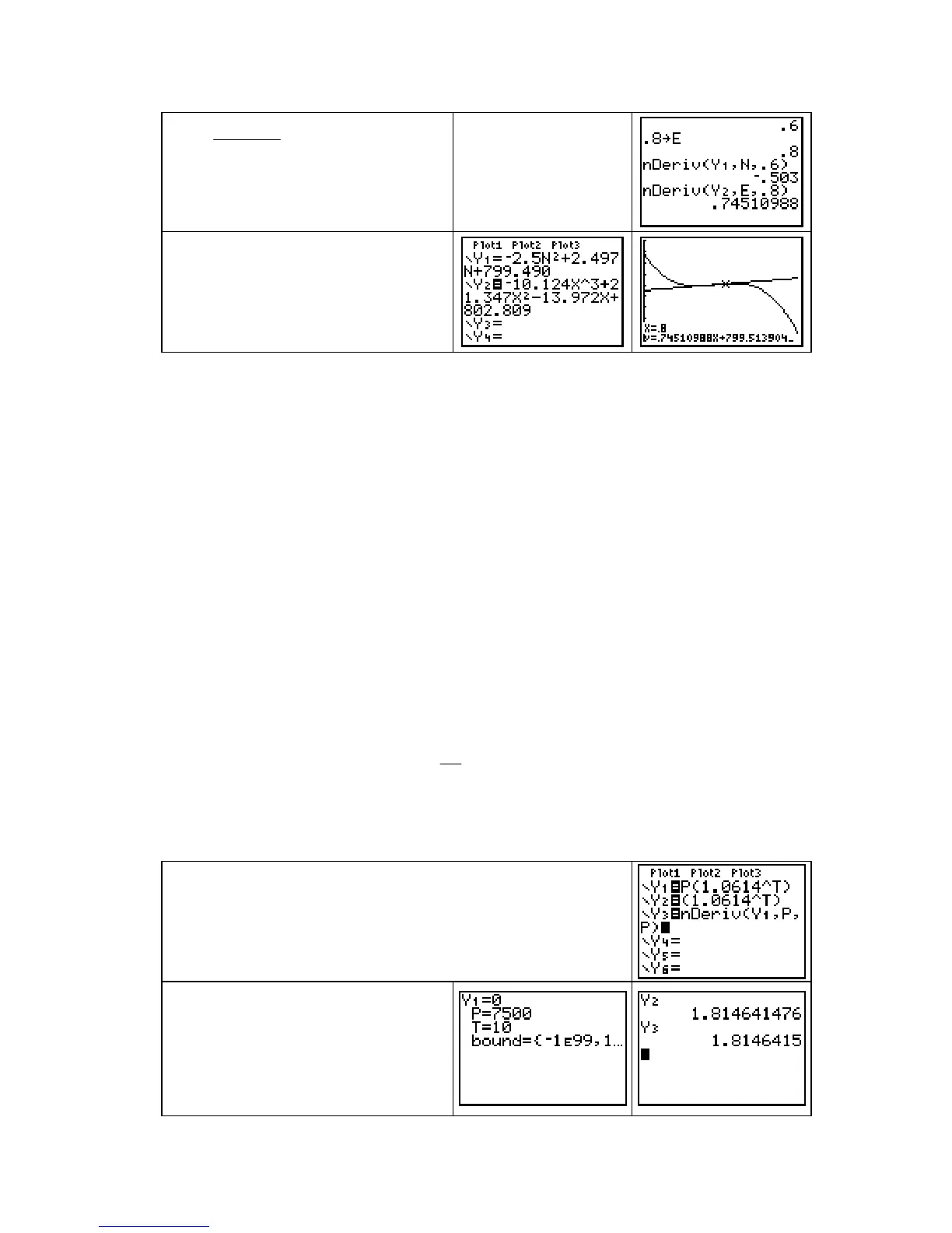
dE e
de
( .6), 0
evaluated at e = 0.8 to
be about 0.745 foot per mile.
(Always remember to attach units of
measure to the numerical values.)
It is not necessary to again
store the values for N and
E unless for some reason
they have been changed.
If you want to see the line tangent to
the graph of
E(e, 0.6) at e = 0.8, first
change
E in Y2 to X and turn off Y1.
Draw the graph and use the
Tangent
instruction in the DRAW menu.
9.3 Partial Rates of Change
When holding all but one of the input variables in a multivariable function constant, you are
actually looking at a function of one input variable. Thus, all of the techniques for finding
derivatives that we discussed previously can be used. In particular, the calculator’s numerical
derivative
nDeriv can be used to find partial rates of change at specific values of the varying
input variable.
Although your calculator does not give formulas for derivatives, you can use it as
discussed on page 58 of this
Guide to check your answer for the algebraic formula for a partial
derivative.
NUMERICALLY CHECKING PARTIAL DERIVATIVE FORMULAS As mentioned in
Chapter 3, the basic concept in checking your algebraically-found partial derivative formula is
that your formula and the calculator's formula computed with
nDeriv should have the same
outputs when each is evaluated at several different randomly-chosen inputs. You can use the
methods on pages 102 and 103 of this
Guide to evaluate each derivative formula at several
different inputs and determine if the same numerical values are obtained from each formula.
We illustrate these ideas by checking the answers for the partial derivative formulas found
in parts
b of Example 1 in Section 9.3 of Calculus Concepts for the following function:
The accumulated value of an investment of
P dollars over t years at an APR of 6%
compounded quarterly is
A(P, t) = P
()
4
0.06
4
11.0
t
t
P+≈614
dollars.
Recall that the syntax for the calculator’s numerical derivative is
nDeriv(function, symbol for input variable, point at which the derivative is evaluated)
Enter the function A, using the letters P and T that appear in the
formula, in
Y1.
Part b of Example 1 asks for a formula for ∂A/∂P, so enter your
formula in
Y2. Enter the calculator’s derivative, using P as the
changing input, in
Y3.
Use the MATH SOLVER to store P
= 7500 and T=10. Go to the home
screen and evaluate Y2 and Y3. If
the outputs of
Y2 and Y3 are the
same, your answer in
Y2 is probably
correct.
Copyright © Houghton Mifflin Company. All rights reserved.
102