Chapter 10
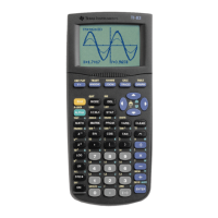
Using equations [1] and [2] on page
109, enter the coefficients of l in the
first column, the coefficients of t in
the second column, and the constant
terms in the third column of matrix
A.
The numbers at the bot-
tom of the screen give the
row and column that is
highlighted. “2, 3” means
that
−
5.3 is in the 2nd row
and the 3rd column.
Return to the home screen. The keystrokes that give the solu-
tion to the system of equations, provided that a solution exists,
are
1
2ND (MATRIX)x
−
► [MATH] ALPHA APPS
[rref(]
1
2ND (MATRIX)x
−
1 [A] ) ENTER . Press and hold
► to view all the digits in the third column.
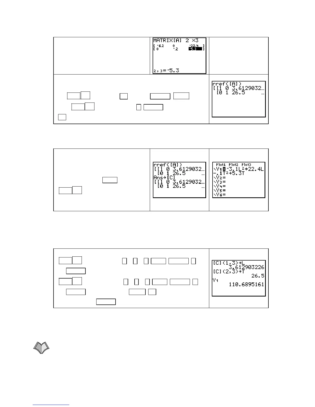
Carefully notice the order in which you entered the coefficients. Because the coefficient of l
was input first in matrix
A, the first value in the third column of the solution is the value of l.
The second value in the third column is the value of
t.
We need to use the unrounded values
of
l and t to find the multivariable
function output at the critical point.
So, store this solution in another
matrix, say
C, with STO`
1
2ND (MATRIX)x
−
3 [C].
Also, enter the multivariable
function
V in Y1.
We illustrate how to recall a particular matrix element so that we can use the unrounded values
of
l and t to find the multivariable function output. Recall that a matrix element is referred to
by the row and then the column in which it appears. Because
C is a 2 by 3 matrix (2 rows and 3
columns) and we set up the equations so that
l is the input variable whose coefficient we
entered first in matrix
A, l is in the (1, 3) position and t is in the (2, 3) position.
On the home screen, store the value of l into L with
1
2ND (MATRIX)x
−
3 [C] ( 1 , 3 ) STO` ALPHA )
(L) ENTER
. Store the value of c into C with
1
2ND (MATRIX)x
−
3 [C] ( 2 , 3 ) STO` ALPHA 4
(T) ENTER
. Find V(l, t) with VARS ► [Y−VARS] 1
[Function] 1 [Y1] ENTER
.
10.3 Optimization Under Constraints
Optimization techniques on your calculator when a constraint is involved are the same as the
ones discussed in Sections 10.2.1a and 10.2.2 except that there is one additional equation in
the system of equations to be solved.
10.3.1 FINDING OPTIMAL POINTS ALGEBRAICALLY AND CLASSIFYING OPTIMAL
POINTS UNDER CONSTRAINED OPTIMIZATION
We illustrate solving a con-
Copyright © Houghton Mifflin Company. All rights reserved.
110

 Loading...