Chapter 5
• The calculator’s fnInt function yields the same result (to 3 decimal places) as that found in
the limit of sums investigation on page 66 of this Guide.
5.3 The Fundamental Theorem of Calculus
Intuitively, this theorem tells us that the derivative of an antiderivative of a function is the
function itself. Let us view this idea both numerically and graphically. The correct syntax for
the calculator’s numerical integrator is
fnInt(function, name of input variable, left endpoint for input, right endpoint for input)
Consider the function f(t) = 3t
2
+ 2t – 5 and the accumulation function F(x) = ftdt
x
()
1
.
The Fundamental Theorem of Calculus tells us that F
′(x) =
d
dx
ftdt
x
()
1
F
H
I
K
= f(x); that is, F ′(x)
is f evaluated at x.
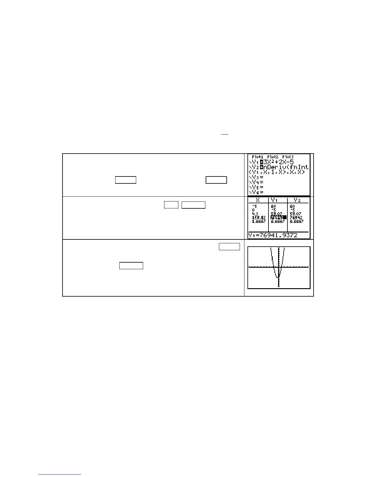
Input f in Y1 and F ′in Y2 (remember that the calculator requires
that you use
X as the input variable in the Y= list).
Access
fnInt with MATH 9 [fnInt(] and nDeriv with MATH 8
[nDeriv(]. (
Turn off any stat plots that are on.)
Have TBLSET set to ASK and press 2ND GRAPH (TABLE).
Input several different values for
X.
Other than occasional roundoff error because the calculator is
approximating these values, the results are identical.
Find a suitable viewing window such as the one set with ZOOM
6 [ZStandard].
Without changing the window (that is, draw the
graphs by pressing
GRAPH ), turn off Y2 and draw the graph of
Y1. Then turn off Y1 and draw the graph of Y2. (Note: The graph
of
Y2 takes a while to draw.) Turn both Y1 and Y2 on and draw
the graph of both functions. Only one graph is seen in each case.
EXPLORE: Enter several other functions in Y1 and do not change Y2 except possibly for the
left endpoint 1 in the
fnInt expression. Perform the same explorations as above. Confirm your
results with derivative and integral formulas.
DRAWING ANTIDERIVATIVE GRAPHS Recall when using fnInt(f(x), x, a, b) that a and
b are, respectively, the lower and upper endpoints of the input interval. Also remember that
you do not have to use x as the input variable unless you are graphing the integral or
evaluating it using the calculator’s table.
Unlike when graphing using
nDeriv, the calculator will not graph a general antiderivative;
it only draws the graph of a specific accumulation function. Thus, we can use x for the input at
the upper endpoint when we want to draw an antiderivative graph, but not for the inputs at
both the upper and lower endpoints.
All of the antiderivatives of a specific function differ only by a constant. We explore this
idea using the function
f(x) = 3x
2
– 1 and its general antiderivative F(x) = x
3
– x + C. Because
we are working with a general antiderivative in this illustration, we do not have a starting point
for the accumulation. We therefore choose some value, say 0, to use as the starting point for
the accumulation function to illustrate drawing antiderivative graphs. If you choose a different
lower limit, your results will differ from those shown below by a constant.
Copyright © Houghton Mifflin Company. All rights reserved.
74

 Loading...


