TI-83, TI-83 Plus, TI-84 Plus Guide
10.3.2 FINDING OPTIMAL POINTS USING MATRICES AND CLASSIFYING OPTIMAL
POINTS UNDER CONSTRAINED OPTIMIZATION
Remember that a matrix solution
method only can be used with a system of linear partial derivative equations. We choose to
illustrate the matrix process of solving with matrix Method 2 (discussed on page 110) for the
sausage production function in Example 3 of Section 10.3 in
Calculus Concepts. The system
of partial derivative equations and the constraint, written with the constant terms on the right-
hand side of the equations and the coefficients of the three input variables in the same
positions on the left-hand side of each equation, is
−
5.83s – λ =
−
1.13 (The order in which the variables appear does not
−
5.83w – λ =
−
1.04 matter as long as it is the same in each equation.)
w + s = 1
When a particular variable does not appear in an equation, its coefficient is zero.
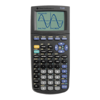
Press
1
2ND (MATRIX)x
−
and then ► ► to go to the EDIT
menu. Press
ENTER . Set the dimensions of matrix A to be 3 by
4 (that is, 3 rows and 4 columns).
Enter the coefficients of
s in the first column, the coefficients of
w in the second column, and the coefficients of λ in the third
column, and the constant terms in the fourth column of matrix
A.
(See the matrix on p. 652 of
Calculus Concepts.)
Return to the home screen. The keystrokes that give the solu-
tion to the system of equations, provided that a solution exists,
are
1
2ND (MATRIX)x
−
► [MATH] ALPHA APPS
[rref(]
1
2ND (MATRIX)x
−
1 [A] ) ENTER . Press and hold
► to view all the digits in the third column.
The solution to the system of equations is s ≈ 0.508, w ≈ 0.492,
and
λ =
−
1.83.
Store this result in matrix
C for use with what follows.
Because a contour graph is given (See Figure 10.24 in the text), it is easiest to use it to verify
that the optimal point is a minimum. However, we show the method of choosing close points
on the constraint to give another example of this method of classification of optimal points.
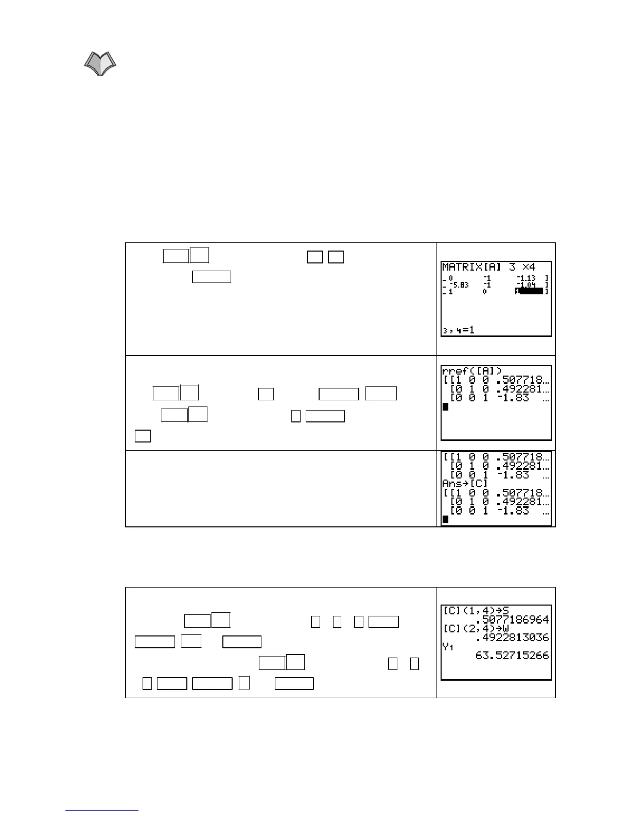
Store the unrounded values of
s ≈ 0.508, w ≈ 0.492, and λ =
−
1.83. Use
1
2ND (MATRIX)x
−
3 [C] ( 1 , 4 ) STO`
ALPHA
LN (S) ENTER to store the value of s in S. Store
the value of
w into W with
1
2ND (MATRIX)x
−
3 [C] ( 2 ,
4 )
STO` ALPHA (W) ENTER . Evaluate Y1. −
We will use the solver with Y2 to find values on the constraint to test against the optimal value
Copyright © Houghton Mifflin Company. All rights reserved.
113

 Loading...