TI-83, TI-83 Plus, TI-84 Plus Guide
Take the derivative of
Y2 = V
h
with respect to h and we have
V
hh
, the partial derivative of V with respect to h and then h
again. Find V
hh
=
−
72 at the critical point.
Take the derivative of
Y3 = V
w
with respect to h and we have
V
wh
, the partial derivative of V with respect to w and then h.
Find V
wh
=
−
36 at the critical point.
If you prefer, enter the value
of H in the 3rd position.
Take the derivative of Y2 = V
h
with respect to w and we have
V
hw
, the partial derivative of V with respect to h and then w.
Find V
hw
=
−
36 at the critical point. (Note: V
wh
must equal V
hw
.)
Take the derivative of
Y3 = V
w
with respect to w and we have
V
ww
, the partial derivative of V with respect to w and then w
again. Find V
ww
=
−
72 at the critical point.
If you prefer, enter the value
of W in the 3rd position.
The second partials matrix is
VV
VV
hh hw
wh ww
M
O
Q
P
. Find the value of
D = (
−
72)(
−
72) – (
−
36)
2
= 3888. Because D > 0 and V
hh
< 0 at
the critical point, the Determinant Test tells us that (h, w, V) =
(18, 18, 11664) is a relative maximum point.
NOTE: The values of the second partial derivatives were not very difficult to determine with-
out the calculator in this example. However, with a more complicated function, we strongly
suggest using the above methods to provide a check on your analytic work to avoid making
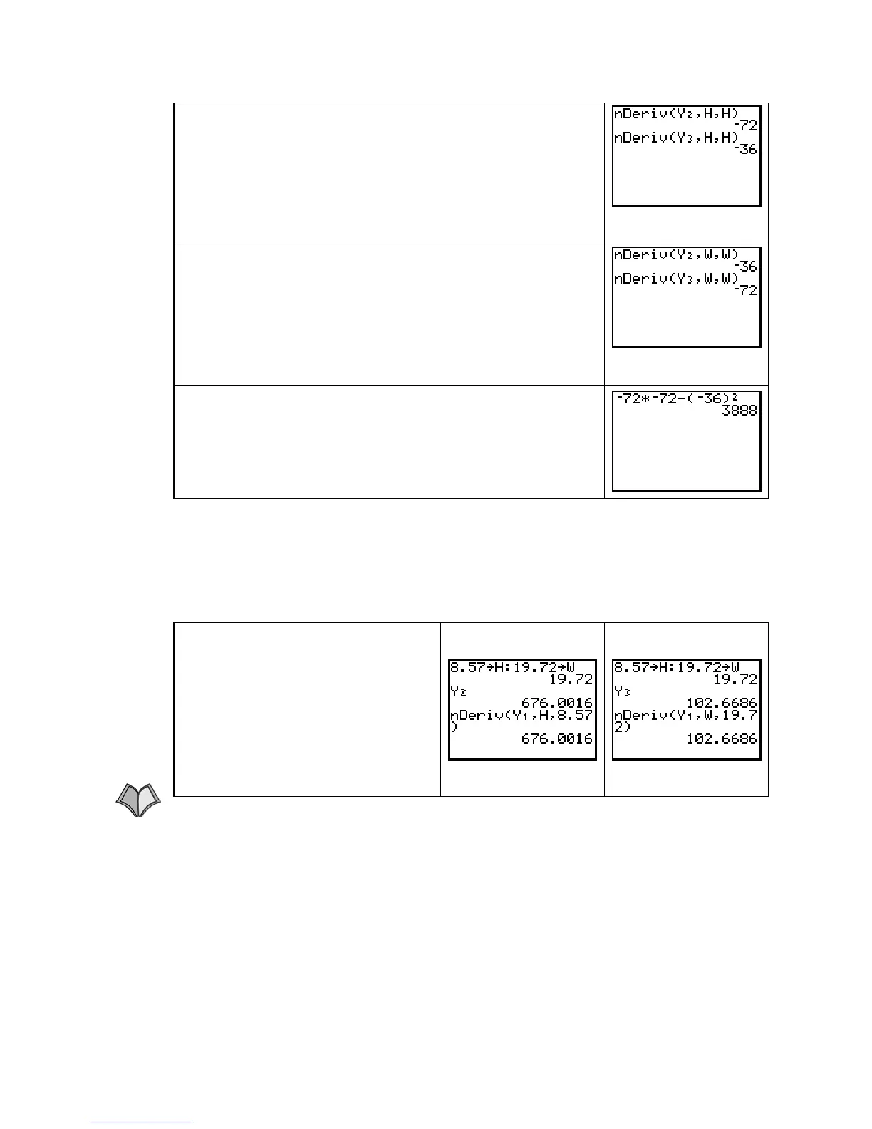
simple mistakes. You can also use the function in
Y1 to check the derivatives in Y2 and Y3.
We use some randomly chosen values of
H and W to illustrate this quick check rather than use
the values at the critical point, because the critical point values give 0 for
Y2 and Y3.
Store different values in H and W and
evaluate
Y2 at these values. Then
evaluate the calculator’s derivative of
Y1 with respect to H at these same
values.
Evaluate
Y3 at these stored values of
H and W. Then evaluate the
calculator’s derivative of
Y1 with
respect to
W at these same values.
10.2.2 FINDING CRITICAL POINTS USING MATRICES To find the critical point(s) of a
smooth, continuous multivariable function, we first find the partial derivatives with respect
to each of the input variables and then set the partial derivatives equal to zero. This gives a
system of equations that needs to be solved. Here we illustrate solving this system using an
orderly array of numbers that is called a matrix.
WARNING: The matrix solution method applies only to linear systems of equations. That
is, the system of equations should not have any variable appearing to a power higher than 1
and should not contain a product of any variables. If the system is not linear, you must use
algebraic solution methods to solve the system. Using your calculator with the algebraic
solution method is illustrated on page 106 of this Guide.
Copyright © Houghton Mifflin Company. All rights reserved.
107

 Loading...