Chapter 6
Enter
fnInt(Y1, X, E, X) in a location of
the
Y= list, say Y3. Turn off Y1 and
Y2. Set the calculator TABLE to ASK
and enter increasingly larger values of
X such as those shown to the right.
It appears that ≈ 4.360, giving social gain ≈ 1.108 + 4.360 ≈ $5.5 million. lim ( )
N
E
N
Dpdp
→∞
z
NOTE: The remainder of the material in this Guide refers to the complete text for Calculus
Concepts (that also contains Section 6.4 and Chapters 7 - 10.)
6.4 Probability Distributions and Density Functions
Most of the applications of probability distributions and density functions use technology tech-
niques that have already been discussed. Probabilities are areas whose values can be found by
integrating the appropriate density function. A cumulative density function is an accumulation
function of a probability density function.
Your calculator’s numerical integrator is especially useful for finding means and standard
deviations of some probability distributions because those integrals often involve expressions
for which we have not developed algebraic techniques for finding antiderivatives. The calcu-
lator contains many built-in statistical menus that deal with probability distributions and
density functions. These are especially useful when you take a statistics course, but some can
be used with Section 6.4 in this course. Consult your Calculator Owners’ Manual for more
details and instructions for use of these features.
NORMAL PROBABILITIES
The normal density function is the most well known and
widely used probability distribution. If you are told that a random variable x has a normal
distribution N(x) with mean
µ
and standard deviation
σ
, the probability that x is between two
real numbers a and b is given by
Nxdx e dx
a
b
a
b
x
()
()
zz
=
−−
1
2
2
2
2
σπ
µ
σ
We illustrate these ideas with the situation in Example 8 of Section 6.4 of Calculus Concepts.
In that example, we are given that the distribution of the life of the bulbs, with the life span
measured in hundreds of hours, is modeled by a normal density function with
µ
= 900 hours
and
σ
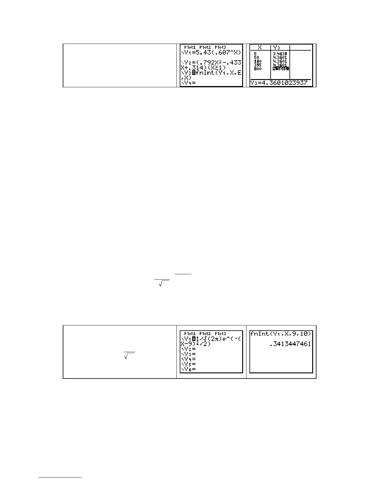
= 100 hours. Carefully use parentheses when entering the normal density function.
The probability that a light bulb lasts
between 9 and 10 hundred hours is
P(9 ≤ x ≤ 10) =
1
2
9
10
92
2
π
−−
ed
x()/
x
The value of this integral must be a
number between 0 and 1.
VIEWING NORMAL PROBABILITIES We could have found the probability that the
light bulb life is between 900 and 1000 hours graphically by using the
CALC menu.
Copyright © Houghton Mifflin Company. All rights reserved.
88

 Loading...