HP 39gs Master Guide

12
T
T
H
H
E
E
E
E
X
X
P
P
E
E
R
R
T
T
:
:
V
V
E
E
C
C
T
T
O
O
R
R
F
F
U
U
N
N
C
C
T
T
I
I
O
O
N
N
S
S
F
F
u
u
n
n
a
a
n
n
d
d
g
g
a
a
m
m
e
e
s
s
Apart from the normal mathematical and engineering applications of parametric equations, some interesting
graphs are available through this aplet. Three quick examples are given below.
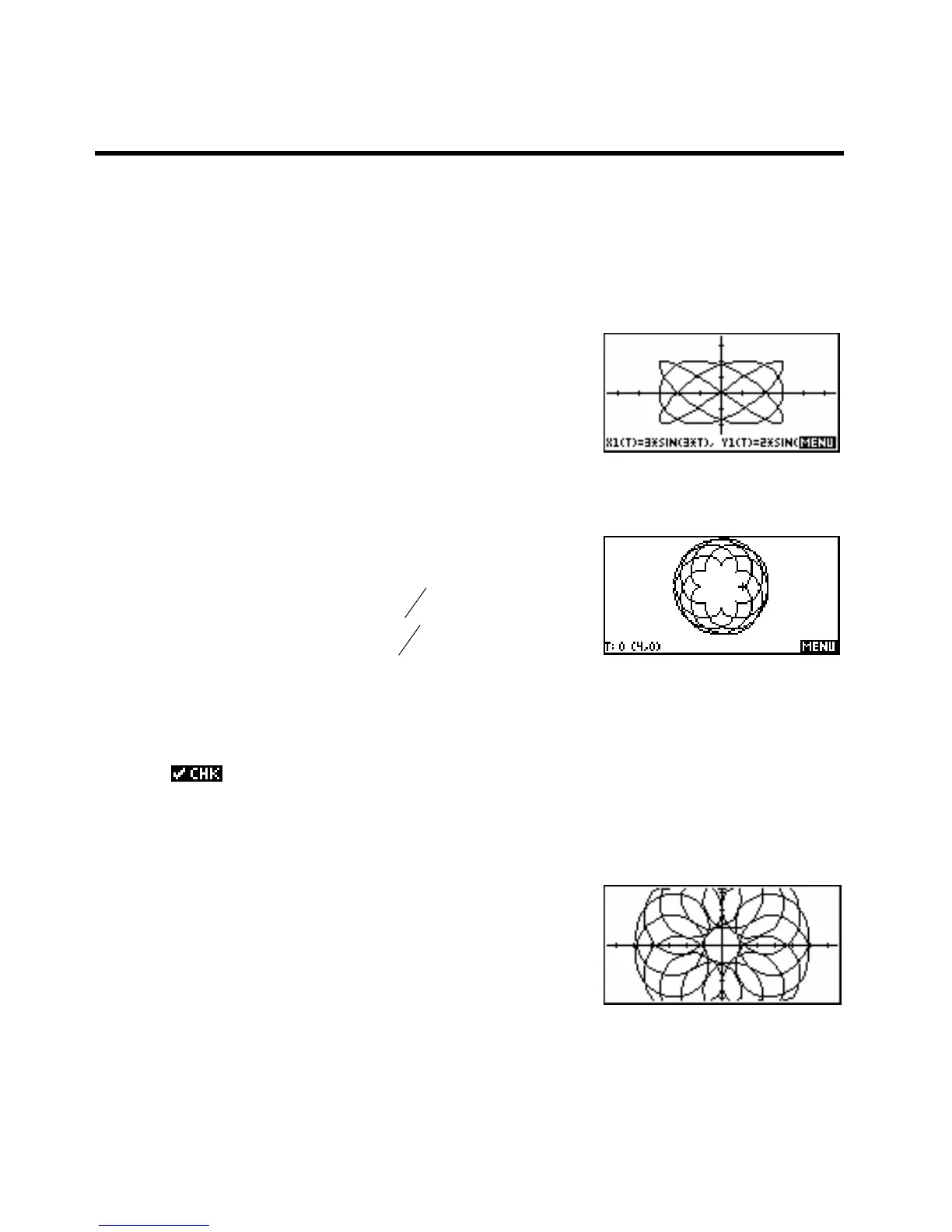
Example 1
Try exploring variants of the graph of:
()
= 3sin 3t
x
t
()
= 2sin 4t yt
Example 2
Try varying the values of A and B in the equations:
+ ) −
x
1(t) = ( A B)cos(t Bcos((
A
t
B
+1) )
1( + ) −
yt
) = (
A B
)sin(
t B
sin((
A
t
B
+1) )
Hint: An easy way to vary A and B is to store values to memories
A and B in the HOME view and enter the
equations exactly as shown. New graphs can then be created by changing back to
HOME and
storing different values to
A and B. The example shown uses A=4, B=2.5 and has axes set with
TRng of 0 to 31.5 step .2, XRng of -21.66 to 21.66 and YRng of -12 to 9. It also has Axes
un-
’d in PLOT SETUP.
Example 2
Try varying the constants in the equations:
x
1(t) =3sin(t) +2sin(15t)
1(
yt) = 3cos(t) +2cos(15t)
For those who remember them, this is curve like those produced by a “Spirograph”.
95

HP 39gs Specifications

General

Type	Scientific
Form factor	Pocket
Product color	Gray
Internal memory	0.256 MB

Weight and Dimensions

Weight	249 g
Dimensions (WxDxH)	187 x 94 x 31 mm